csci5607/exam-2/exam2.md

geometry	output	title	subtitle	date	author
margin=2cm	pdf_document	Exam 2	CSCI 5607	\today	| Michael Zhang | zhan4854@umn.edu $\cdot$ ID: 5289259

\renewcommand{\c}[1]{\textcolor{gray}{#1}} \renewcommand{\r}[1]{\textcolor{red}{#1}} \newcommand{\now}[1]{\textcolor{blue}{#1}} \newcommand{\todo}[0]{\textcolor{red}{\textbf{TODO}}}

Reflection and Refraction

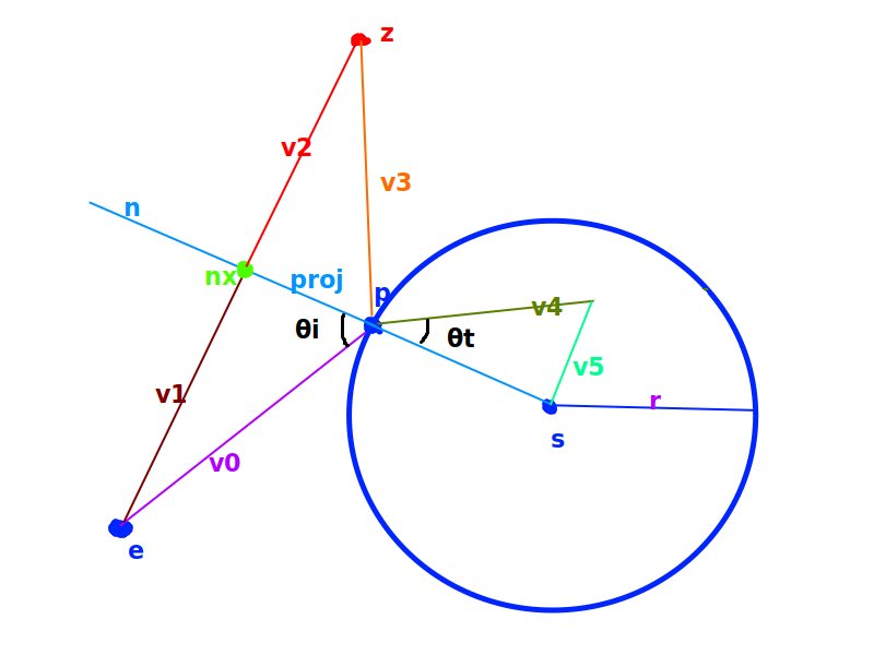
1. \c{Consider a sphere S made of solid glass (\eta = 1.5) that has radius r = 3 and is centered at the location s = (2, 2, 10) in a vaccum ($\eta = 1.0$). If a ray emanating from the point e = (0, 0, 0) intersects S at a point p = (1, 4, 8):}

   Legend for the rest of the problem:

   {width=50%}

   a. \c{(2 points) What is the angle of incidence \theta_i?}

   The incoming ray is in the direction I = v_0 = p - e = (1, 4, 8), and the normal at that point is:

   • N = p - s = (1, 4, 8) - (2, 2, 10) = (-1, 2, -2)

   The angle can be found by taking the opposite of the incoming ray -I and using the formula:

   • $\cos \theta_i = \frac{-I \cdot N}{|I|_2 |N|_2} = \frac{(-1, -4, -8) \cdot (-1, 2, -2)}{9 \cdot 3} = \frac{1 - 8 + 16}{27} = \frac{1}{3}$.

   So the angle \boxed{\theta_i = \cos^{-1}\left(\frac{1}{3}\right)}.

   b. \c{(1 points) What is the angle of reflection \theta_r?}

   The angle of reflection always equals the angle of incidence, $\theta_r = \theta_i = \boxed{\cos^{-1}\left(\frac{1}{3}\right)}$.

   c. \c{(3 points) What is the direction of the reflected ray?}

   The reflected ray can be found by first projecting the incident ray v_0 onto the normalized normal n, which is:

   • proj = n \times |v_0|\cos(\theta_i) = \left(\frac{1}{3}, -\frac{2}{3}, \frac{2}{3}\right) \times 9 \times \frac{1}{3} = (-1, 2, -2)

   Then, we know the point on N where this happened is:

   • nx = p + proj = (1, 4, 8) + (-1, 2, -2) = (0, 6, 6).

   Now, we can subtract this point from where the ray originated to know the direction to add in the other direction, which is still (0, 6, 6) in this case since the ray starts at the origin. Adding this to the point nx gets us (0, 12, 12), which means a point from the origin will get reflected to (0, 12, 12).

   Finally, subtract the point to get the final answer $(0, 12, 12) - (1, 4, 8) = \boxed{(-1, 8, 4)}$.

   d. \c{(3 points) What is the angle of transmission \theta_t?}

   Using Snell's law, we know that

   \begin{align} \eta_i \sin \theta_i &= \eta_t \sin \theta_t \ \r{1.0} \times \sin \theta_i &= \r{1.5} \times \sin \theta_t \ 1.0 \times \sin(\r{ \cos^{-1}(-\frac{1}{3}) }) &= 1.5 \times \sin \theta_t \ 1.0 \times \r{ \frac{2\sqrt{2}}{3} } &= 1.5 \times \sin \theta_t \ \r{ \frac{1.0}{1.5} } \times \frac{2\sqrt{2}}{3} &= \sin \theta_t \ \r{ \frac{4}{9} } \sqrt{2} &= \sin \theta_t \ \theta_t &= \sin^{-1} \left(\frac{4}{9}\sqrt{2}\right) \approx \boxed{0.67967 \ldots} \end{align}

   e. \c{(4 points) What is the direction of the transmitted ray?}

   We can just add together s - p and v_5 in the diagram above, these two make up the orthogonal basis of the transmitted ray v_4. The lengths of these two are not important, but related through the angle \theta_t.

   Also note that in the diagram, the sphere is drawn as a 2D circle. But in reality, the number of vectors perpendicular to s - p is infinite. The v_5 we're looking for is parallel with v_1, so we can just use \frac{v_1}{\|v_1\|_2} as our unit vector for v_5.

   \begin{align} v_4 &= (s - p) + \tan \theta_t \times |s - p|_2 \times \frac{v_1}{|v_1|_2} \ v_4 &= (\r{ (2, 2, 10) - (1, 4, 8) }) + \tan \theta_t \times |s - p|_2 \times \frac{v_1}{|v_1|_2} \ v_4 &= \r{ (1, -2, 2) } + \tan \theta_t \times |\r{(1, -2, 2)}|_2 \times \frac{v_1}{|v_1|_2} \ v_4 &= (1, -2, 2) + \tan \theta_t \times \r{3} \times \frac{v_1}{|v_1|_2} \ v_4 &= (1, -2, 2) + \tan \theta_t \times 3 \times \frac{\r{(0, 6, 6)}}{|\r{(0, 6, 6)}|_2} \ v_4 &= (1, -2, 2) + \tan \theta_t \times 3 \times \r{\left(0, \frac{\sqrt{2}}{2}, \frac{\sqrt{2}}{2}\right)} \ v_4 &= (1, -2, 2) + \tan \theta_t \times \left(0, \r{\frac{3}{2}\sqrt{2}}, \r{\frac{3}{2}\sqrt{2}} \right) \ v_4 &= (1, -2, 2) + \r{\frac{4}{7}\sqrt{2}} \times \left(0, \frac{3}{2}\sqrt{2}, \frac{3}{2}\sqrt{2} \right) \ v_4 &= (1, -2, 2) + \r{\left(0, \frac{12}{7}, \frac{12}{7} \right)} \ v_4 &= \r{\left(1, \frac{-2}{7}, \frac{26}{7} \right)} \ \end{align}

   This can be normalized into $\boxed{\left(\frac{7}{27}, -\frac{2}{27}, \frac{26}{27}\right)}$.

Geometric Transformations

2. \c{(8 points) Consider the airplane model below, defined in object coordinates with its center at (0, 0, 0), its wings aligned with the $\pm x$ axis, its tail pointing upwards in the +y direction and its nose facing in the +z direction. Derive a sequence of model transformation matrices that can be applied to the vertices of the airplane to position it in space at the location p = (4, 4, 7), with a direction of flight $w = (2, 1, -2)$ and the wings aligned with the direction d = (-2, 2, -1).}

   There's 2 discrete transformations going on here:

   • First, we must rotate the plane. Since we are given orthogonal directions for the flight and wings, we can just come up with another vector for the tail direction by doing:

     y' = (2, 1, -2) \times (-2, 2, -1) = (1, 2, 2)

     Now we can construct a 3D rotation matrix:

     $$ R = \begin{bmatrix} d_x & y_x & w_x & 0 \ d_y & y_y & w_y & 0 \ d_z & y_z & w_z & 0 \ 0 & 0 & 0 & 1 \end{bmatrix}

     \begin{bmatrix} -2 & 1 & 2 & 0 \ 2 & 2 & 1 & 0 \ -1 & 2 & -2 & 0 \ 0 & 0 & 0 & 1 \end{bmatrix}

   • Now we just need to translate this to the position (4, 4, 7). This is easy with:

     $$ T = \begin{bmatrix} 1 & 0 & 0 & 4 \ 0 & 1 & 0 & 4 \ 0 & 0 & 1 & 7 \ 0 & 0 & 0 & 1 \ \end{bmatrix}

   We can just compose these two matrices together (by doing the rotation first, then translating!)

   $$ TR = \begin{bmatrix} -2 & 1 & 2 & 4 \ 2 & 2 & 1 & 4 \ -1 & 2 & -2 & 7 \ 0 & 0 & 0 & 1 \end{bmatrix}

3. \c{Consider the earth model shown below, which is defined in object coordinates with its center at (0, 0, 0), the vertical axis through the north pole aligned with the direction (0, 1, 0), and a horizontal plane through the equator that is spanned by the axes (1, 0, 0) and (0, 0, 1).}

   a. \c{(3 points) What model transformation matrix could you use to tilt the vertical axis of the globe by 23.5^\circ away from (0, 1, 0), to achieve the pose shown in the image on the right?}

   You could use a 3D rotation matrix. Since the axis of rotation is the $z$-axis, the rotation matrix would look like:

   $$ M_1 = \begin{bmatrix} \cos(23.5^\circ) & \sin(23.5^\circ) & 0 & 0 \ -\sin(23.5^\circ) & \cos(23.5^\circ) & 0 & 0 \ 0 & 0 & 1 & 0 \ 0 & 0 & 0 & 1 \ \end{bmatrix}

   b. \c{(5 points) What series of rotation matrices could you apply to the globe model to make it spin about its tilted axis of rotation, as suggested in the image on the right?}

   One way would be to rotate it back to its normal orientation, apply the spin by whatever angle \theta(t) it was spinning at at time t, and then put it back into its 23.5^\circ orientation. This rotation is done around the $y$-axis, so the matrix looks like:

   $$ M_2 = M_1^{-1} \begin{bmatrix} \cos(\theta(t)) & 0 & \sin(\theta(t)) & 0 \ 0 & 1 & 0 & 0 \ -\sin(\theta(t)) & 0 & \cos(\theta(t)) & 0 \ 0 & 0 & 0 & 1 \ \end{bmatrix} M_1

   c. \c{[5 points extra credit] What series of rotation matrices could you use to send the tilted, spinning globe model on a circular orbit of radius $r$ around the point (0, 0, 0) within the xz plane, as illustrated below?}

   In the image, the globe itself does not rotate, but I'm going to assume it revolves around the sun at a different angle \phi(t). The solution here would be to rotate the globe after the translation to whatever its position is.

   • First, rotate the globe to the 23.5^\circ tilt, using M_2 as described above.

   • Then, translate the globe to its position, which I'm going to assume is (r, 0, 0).

     $$ M_3 = \begin{bmatrix} 1 & 0 & 0 & r \ 0 & 1 & 0 & 0 \ 0 & 0 & 1 & 0 \ 0 & 0 & 0 & 1 \ \end{bmatrix}

   • Finally, rotate by \phi(t) around the $y$-axis after the translation, using:

     $$ M_4 = \begin{bmatrix} \cos(\phi(t)) & 0 & \sin(\phi(t)) & r \ 0 & 1 & 0 & 0 \ -\sin(\phi(t)) & 0 & \cos(\phi(t)) & 0 \ 0 & 0 & 0 & 1 \ \end{bmatrix}

   The resulting transformation matrix is M = \boxed{M_4 M_3 M_2}.

The Camera/Viewing Transformation

4. \c{Consider the viewing transformation matrix V that enables all of the vertices in a scene to be expressed in terms of a coordinate system in which the eye is located at (0, 0, 0), the viewing direction ($-n$) is aligned with the -z axis (0, 0, -1), and the camera's 'up' direction (which controls the roll of the view) is aligned with the y axis (0, 1, 0).}

   a. \c{(4 points) When the eye is located at e = (2, 3, 5), the camera is pointing in the direction (1, -1, -1), and the camera's 'up' direction is (0, 1, 0), what are the entries in V?}

   • Viewing direction is (1, -1, -1).
   • Normalized n = (\frac{1}{\sqrt{3}}, -\frac{1}{\sqrt{3}}, -\frac{1}{\sqrt{3}}).
   • u = up \times n = (\frac{1}{\sqrt{2}}, 0, \frac{1}{\sqrt{2}}).
   • v = n \times u = (\frac{\sqrt{6}}{6}, \frac{2}{\sqrt{6}}, -\frac{\sqrt{6}}{6})
   • d_x = - (eye \cdot u) = - (2 \times \frac{1}{\sqrt{2}} + 5 \times \frac{1}{\sqrt{2}}) = -\frac{7}{\sqrt{2}}
   • $d_y = - (eye \cdot v) = - (2 \times \frac{1}{\sqrt{6}} + 3 \times \frac{2}{\sqrt{6}} - 5 \times \frac{1}{\sqrt{6}}) = -\frac{3}{\sqrt{6}}$
   • $d_z = - (eye \cdot n) = - (2 \times \frac{1}{\sqrt{3}} - 3 \times \frac{1}{\sqrt{3}} - 5 \times \frac{1}{\sqrt{3}}) = -\frac{6}{\sqrt{3}}$

   $$ \begin{bmatrix} \frac{1}{\sqrt{2}} & 0 & \frac{1}{\sqrt{2}} & -\frac{7}{\sqrt{2}} \ \frac{1}{\sqrt{6}} & \frac{2}{\sqrt{6}} & -\frac{1}{\sqrt{6}} & -\frac{3}{\sqrt{6}} \ -\frac{1}{\sqrt{3}} & \frac{1}{\sqrt{3}} & \frac{1}{\sqrt{3}} & -\frac{6}{\sqrt{3}} \ 0 & 0 & 0 & 1 \ \end{bmatrix}

   Also solved using a Python script:

   def view_matrix(camera_pos, view_dir, up_dir):
     n = unit(-view_dir)
     u = unit(np.cross(up_dir, n))
     v = np.cross(n, u)
     return np.array([
       [u[0], u[1], u[2], -np.dot(camera_pos, u)],
       [v[0], v[1], v[2], -np.dot(camera_pos, v)],
       [n[0], n[1], n[2], -np.dot(camera_pos, n)],
       [0, 0, 0, 1],
     ])
   
   camera_pos = np.array([2, 3, 5])
   view_dir = np.array([1, -1, -1])
   up_dir = np.array([0, 1, 0])
   V = view_matrix(camera_pos, view_dir, up_dir)
   print(V)
   

   b. \c{(2 points) How will this matrix change if the eye moves forward in the direction of view? [which elements in V will stay the same? which elements will change and in what way?]}

   If the eye moves forward, the eye position and everything that depends on it will change, while everything else doesn't.

   n	u	v	d
   same	same	same	different

   The n is the same because the viewing direction does not change.

   c. \c{(2 points) How will this matrix change if the viewing direction spins in the clockwise direction around the camera's 'up' direction? [which elements in V will stay the same? which elements will change and in what way?]}

   In this case, the eye position stays the same, and everything else changes.

   n	u	v	d
   different	different	different	same

   d. \c{(2 points) How will this matrix change if the viewing direction rotates directly upward, within the plane defined by the viewing and 'up' directions? [which elements in V will stay the same? which elements will change and in what way?]}

   In this case, the eye position stays the same, and everything else changes.

   n	u	v	d
   different	different	different	same

5. \c{Suppose a viewer located at the point (0, 0, 0) is looking in the $-z$ direction, with no roll ['up' = $(0, 1 ,0)$], towards a cube of width 2, centered at the point (0, 0, -5), whose sides are colored: red at the plane x = 1, cyan at the plane x = -1, green at the plane y = 1, magenta at the plane y = -1, blue at the plane z = -4, and yellow at the plane $z = -6$.}

   a. \c{(1 point) What is the color of the cube face that the user sees?}

   \boxed{\textrm{Blue}}

   b. \c{(3 points) Because the eye is at the origin, looking down the -z axis with 'up' = (0,1,0), the viewing transformation matrix V in this case is the identity I. What is the model matrix M that you could use to rotate the cube so that when the image is rendered, it shows the red side of the cube?}

   You would have to do a combination of (1) translate to the origin, (2) rotate around the origin, and then (3) untranslate back. This way, the eye position doesn't change.

   $$ M = \begin{bmatrix} 1 & 0 & 0 & 0 \ 0 & 1 & 0 & 0 \ 0 & 0 & 1 & -5 \ 0 & 0 & 0 & 1 \ \end{bmatrix} \cdot \begin{bmatrix} 0 & 0 & -1 & 0 \ 0 & 1 & 0 & 0 \ 1 & 0 & 0 & 0 \ 0 & 0 & 0 & 1 \ \end{bmatrix} \cdot \begin{bmatrix} 1 & 0 & 0 & 0 \ 0 & 1 & 0 & 0 \ 0 & 0 & 1 & 5 \ 0 & 0 & 0 & 1 \ \end{bmatrix}

   \boxed{\begin{bmatrix} 0 & 0 & -1 & -5 \ 0 & 1 & 0 & 0 \ 1 & 0 & 0 & -5 \ 0 & 0 & 0 & 1 \ \end{bmatrix}}

   To verify this, testing with an example point (1, 1, -4) yields:

   $$ \begin{bmatrix} 0 & 0 & -1 & -5 \ 0 & 1 & 0 & 0 \ 1 & 0 & 0 & -5 \ 0 & 0 & 0 & 1 \ \end{bmatrix} \cdot \begin{bmatrix} 1 \ 1 \ -4 \ 1 \end{bmatrix}

   \begin{bmatrix} -1 \ 1 \ -4 \ 1 \end{bmatrix}

   c. \c{(4 points) Suppose now that you want to leave the model matrix M as the identity. What is the viewing matrix V that you would need to use to render an image of the scene from a re-defined camera configuration so that when the scene is rendered, it shows the red side of the cube? Where is the eye in this case and in what direction is the camera looking?}

   For this, a different eye position will have to be used. Instead of looking from the origin, you could view it from the red side, and then change the direction so it's still pointing at the cube.

   • eye is located at (5, 0, -5)
   • viewing direction is (-1, 0, 0)
   • n = (1, 0, 0)
   • u = up \times n = (0, 0, -1)
   • v = n \times u = (0, 1, 0)
   • d = (-5, 0, -5)

   The final viewing matrix is $\boxed{\begin{bmatrix} 0 & 0 & -1 & -5 \ 0 & 1 & 0 & 0 \ 1 & 0 & 0 & -5 \ 0 & 0 & 0 & 1 \ \end{bmatrix}}$. Turns out it's the same matrix! Wow!

The Projection Transformation

6. \c{Consider a cube of width 2\sqrt{3} centered at the point $(0, 0, -3\sqrt{3})$, whose faces are colored light grey on the top and bottom $(y = \pm\sqrt{3})$, dark grey on the front and back (z = -2\sqrt{3} and $z = -4\sqrt{3}$), red on the right (x = \sqrt{3}), and green on the left $(x = -\sqrt{3})$.}

   a. \c{Show how you could project the vertices of this cube to the plane $z = 0$ using an orthographic parallel projection:}

   i) \c{(2 points) Where will the six vertex locations be after such a projection, omitting the normalization step?}

   • [\begin{matrix}- \sqrt{3} & - \sqrt{3} & - 4 \sqrt{3}\end{matrix}] \rightarrow [\begin{matrix}-1 & -1 & 7\end{matrix}]
   • [\begin{matrix}- \sqrt{3} & \sqrt{3} & - 4 \sqrt{3}\end{matrix}] \rightarrow [\begin{matrix}-1 & 1 & 7\end{matrix}]
   • [\begin{matrix}\sqrt{3} & - \sqrt{3} & - 4 \sqrt{3}\end{matrix}] \rightarrow [\begin{matrix}1 & -1 & 7\end{matrix}]
   • [\begin{matrix}\sqrt{3} & \sqrt{3} & - 4 \sqrt{3}\end{matrix}] \rightarrow [\begin{matrix}1 & 1 & 7\end{matrix}]
   • [\begin{matrix}- \sqrt{3} & - \sqrt{3} & - 2 \sqrt{3}\end{matrix}] \rightarrow [\begin{matrix}-1 & -1 & 5\end{matrix}]
   • [\begin{matrix}- \sqrt{3} & \sqrt{3} & - 2 \sqrt{3}\end{matrix}] \rightarrow [\begin{matrix}-1 & 1 & 5\end{matrix}]
   • [\begin{matrix}\sqrt{3} & - \sqrt{3} & - 2 \sqrt{3}\end{matrix}] \rightarrow [\begin{matrix}1 & -1 & 5\end{matrix}]
   • [\begin{matrix}\sqrt{3} & \sqrt{3} & - 2 \sqrt{3}\end{matrix}] \rightarrow [\begin{matrix}1 & 1 & 5\end{matrix}]

   ii) \c{(1 points) Sketch the result, being as accurate as possible and labeling the colors of each of the visible faces.}

   This is just a square with the dark gray side facing the camera. The other sides are not visible because the cube is parallel to the axis, and when you do an orthographic projection, those faces are lost.

   {width=40%}

   iii) \c{(2 points) Show how you could achieve this transformation using one or more matrix multiplication operations. Specify the matrix entries you would use, and, if using multiple matrices, the order in which they would be multiplied.}

   Actually, I got the numbers above by using the three transformation matrices in this Python script:

   def ortho_transform(left, right, bottom, top, near, far):
     step_1 = np.array([
       [1, 0, 0, 0],
       [0, 1, 0, 0],
       [0, 0, -1, 0],
       [0, 0, 0, 1],
     ])
   
     step_2 = np.array([
       [1, 0, 0, -((left + right) / 2)],
       [0, 1, 0, -((bottom + top) / 2)],
       [0, 0, 1, -((near + far) / 2)],
       [0, 0, 0, 1],
     ])
   
     step_3 = np.array([
       [(2 / (right - left)), 0, 0, 0],
       [0, (2 / (top - bottom)), 0, 0],
       [0, 0, (2 / (far - near)), 0],
       [0, 0, 0, 1],
     ])
   
     return step_3 @ step_2 @ step_1
   

   b. \c{Show how you could project the vertices of this cube to the plane $z = 0$ using an oblique parallel projection in the direction $d = (1, 0, \sqrt{3})$:}

   i) \c{(3 points) Where will the six vertex locations be after such a projection, omitting the normalization step?}

   • [\begin{matrix}- \sqrt{3} & - \sqrt{3} & - 4 \sqrt{3}\end{matrix}] \rightarrow [\begin{matrix}- \frac{4 \sqrt{3}}{3} - 1 & -1 & 7\end{matrix}]
   • [\begin{matrix}- \sqrt{3} & \sqrt{3} & - 4 \sqrt{3}\end{matrix}] \rightarrow [\begin{matrix}- \frac{4 \sqrt{3}}{3} - 1 & 1 & 7\end{matrix}]
   • [\begin{matrix}\sqrt{3} & - \sqrt{3} & - 4 \sqrt{3}\end{matrix}] \rightarrow [\begin{matrix}1 - \frac{4 \sqrt{3}}{3} & -1 & 7\end{matrix}]
   • [\begin{matrix}\sqrt{3} & \sqrt{3} & - 4 \sqrt{3}\end{matrix}] \rightarrow [\begin{matrix}1 - \frac{4 \sqrt{3}}{3} & 1 & 7\end{matrix}]
   • [\begin{matrix}- \sqrt{3} & - \sqrt{3} & - 2 \sqrt{3}\end{matrix}] \rightarrow [\begin{matrix}- \frac{2 \sqrt{3}}{3} - 1 & -1 & 5\end{matrix}]
   • [\begin{matrix}- \sqrt{3} & \sqrt{3} & - 2 \sqrt{3}\end{matrix}] \rightarrow [\begin{matrix}- \frac{2 \sqrt{3}}{3} - 1 & 1 & 5\end{matrix}]
   • [\begin{matrix}\sqrt{3} & - \sqrt{3} & - 2 \sqrt{3}\end{matrix}] \rightarrow [\begin{matrix}1 - \frac{2 \sqrt{3}}{3} & -1 & 5\end{matrix}]
   • [\begin{matrix}\sqrt{3} & \sqrt{3} & - 2 \sqrt{3}\end{matrix}] \rightarrow [\begin{matrix}1 - \frac{2 \sqrt{3}}{3} & 1 & 5\end{matrix}]

   ii) \c{(2 points) Sketch the result, being as accurate as possible and labeling the colors of each of the visible faces.}

   {width=40%}

   Excuse the poor sketch but the point is the transformation exposes the green face to the left by doing a shear first.

   iii) \c{(4 points) Show how you could achieve this transformation using one or more matrix multiplication operations. Specify the matrix entries you would use, and, if using multiple matrices, the order in which they would be multiplied.}

   It's the same as the ortho, except it uses an extra matrix that is applied before any of the other transformations:

   def oblique_transform(left, right, bottom, top, near, far):
     step_0 = np.array([
       [1, 0, (1 / sqrt3), 0],
       [0, 1, 0, 0],
       [0, 0, 1, 0],
       [0, 0, 0, 1],
     ])
   
     M_ortho = ortho_transform(left, right, bottom, top, near, far)
   
     return M_ortho @ step_0
   

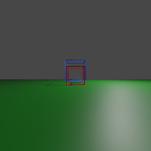
7. \c{Consider the simple scene shown in the image below, where two cubes, one of height 1 and one of height 2, are both resting on a horizontal groundplane ($y = -\frac{1}{2}$), with the smaller cube’s front face aligned with $z = -4$ and the larger cube’s front face aligned with z = -7.}

   a. \c{(5 points) Let the camera location be (0, 0, 0), looking down the $-z$ axis, with the field of view set at 90^\circ. Determine the points, in the image plane, to which each of the cube vertices will be projected and sketch the result to scale. Please clearly label the coordinates to avoid ambiguity.}

   For this part, I reimplemented the perspective rendering algorithm using Python.

   def perspective_matrix(left, right, bottom, top, near, far):
     return np.array([
       [2.0 * near / (right - left), 0, (right + left) / (right - left), 0],
       [0, 2.0 * near / (top - bottom), (top + bottom) / (top - bottom), 0],
       [0, 0, -(far + near) / (far - near), -(2.0 * far * near) / (far - near)],
       [0, 0, -1, 0],
     ])
   
   def view_matrix(camera_pos, view_dir, up_dir):
     n = unit(-view_dir)
     u = unit(np.cross(up_dir, n))
     v = np.cross(n, u)
     return np.array([
       [u[0], u[1], u[2], -np.dot(camera_pos, u)],
       [v[0], v[1], v[2], -np.dot(camera_pos, v)],
       [n[0], n[1], n[2], -np.dot(camera_pos, n)],
       [0, 0, 0, 1],
     ])
   

   The perspective and view matrices are:

   $$ PV = \begin{bmatrix} 1.0 & 0.0 & 0.0 & 0.0 \ 0.0 & 1.0 & 0.0 & 0.0 \ 0.0 & 0.0 & -1.2222 & -2.2222 \ 0.0 & 0.0 & -1.0 & 0.0 \ \end{bmatrix} \begin{bmatrix} 1.0 & 0.0 & 0.0 & -0.0 \ 0.0 & 1.0 & 0.0 & -0.0 \ 0.0 & 0.0 & 1.0 & -0.0 \ 0.0 & 0.0 & 0.0 & 1.0 \ \end{bmatrix}

   Then I ran the transformation using the data given in this particular scene:

   def compute_view(near, vfov, hfov):
     left = -math.tan(hfov / 2.0) * near
     right = math.tan(hfov / 2.0) * near
     bottom = -math.tan(vfov / 2.0) * near
     top = math.tan(vfov / 2.0) * near
     return left, right, bottom, top
   
   def solve(camera_pos, angle):
     angle_radians = math.radians(angle)
     near = 1
     far = 10
     view_dir = np.array([0, 0, -1])
     up_dir = np.array([0, 1, 0])
     left, right, bottom, top = compute_view(near, angle_radians, angle_radians)
     P = perspective_matrix(left, right, bottom, top, near, far)
     V = view_matrix(camera_pos, view_dir, up_dir)
     return P @ V
   
   camera_pos = np.array([0, 0, 0])
   angle = 90
   m = np.around(solve(camera_pos, angle), 4)
   

   This performed the transformation on the front face of the small cube:

   • [\begin{matrix}0.5 & 0.5 & -4.0\end{matrix}] \rightarrow [\begin{matrix}0.5 & 0.5 & 2.6666\end{matrix}]
   • [\begin{matrix}0.5 & -0.5 & -4.0\end{matrix}] \rightarrow [\begin{matrix}0.5 & -0.5 & 2.6666\end{matrix}]
   • [\begin{matrix}-0.5 & -0.5 & -4.0\end{matrix}] \rightarrow [\begin{matrix}-0.5 & -0.5 & 2.6666\end{matrix}]
   • [\begin{matrix}-0.5 & 0.5 & -4.0\end{matrix}] \rightarrow [\begin{matrix}-0.5 & 0.5 & 2.6666\end{matrix}]

   and this transformation on the front face of the large cube:

   • [\begin{matrix}1.0 & 1.5 & -7.0\end{matrix}] \rightarrow [\begin{matrix}1.0 & 1.5 & 6.3332\end{matrix}]
   • [\begin{matrix}1.0 & -0.5 & -7.0\end{matrix}] \rightarrow [\begin{matrix}1.0 & -0.5 & 6.3332\end{matrix}]
   • [\begin{matrix}-1.0 & -0.5 & -7.0\end{matrix}] \rightarrow [\begin{matrix}-1.0 & -0.5 & 6.3332\end{matrix}]
   • [\begin{matrix}-1.0 & 1.5 & -7.0\end{matrix}] \rightarrow [\begin{matrix}-1.0 & 1.5 & 6.3332\end{matrix}]

   Here's a render using Blender:

   {width=40%}

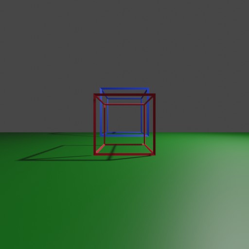
   b. \c{(4 points) How would the image change if the camera were moved forward by 2 units, leaving all of the other parameter settings the same? Determine the points, in the image plane, to which each of the cube vertices would be projected in this case and sketch the result to scale. Please clearly label the coordinates to avoid ambiguity.}

   Here is the updated Blender render:

   {width=40%}

   As you can see, the cubes now take up more of the frame, and in particular the red cube has been warped to take up more camera width than the blue.

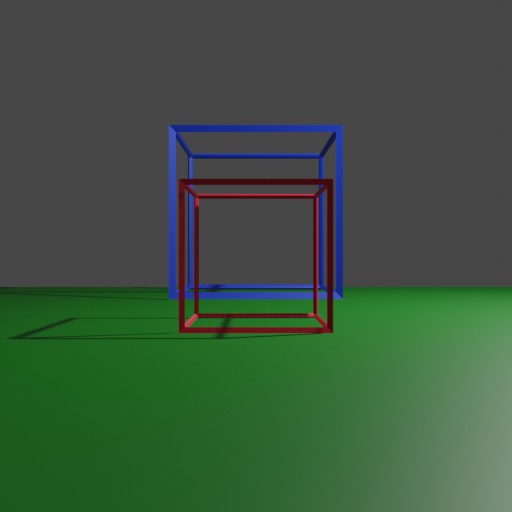
   c. \c{(4 points) How would the image change if, instead of moving the camera, the field of view were reduced by half, to 45^\circ, leaving all of the other parameter settings the same? Determine the points, in the image plane, to which each of the cube vertices would be projected and sketch the result to scale. Please clearly label the coordinates to avoid ambiguity.}

   Here is the updated Blender render:

   {width=40%}

   Because of the reduced FOV, there is less of the scene shown so the cubes take up more of the view. However, there is less of the perspective foreshortening effect, so the front cube doesn't get warped into being wider or bigger than the back cube.

   d. (2 points)

   • \c{Briefly describe what you notice.}

     The cubes aren't warped except when they change distance from the eye.

   • \c{When looking at two cube faces that are equal sizes in reality (e.g. front and back) does one appear smaller than the other when one is more distant from the camera than the other?}

     Yes.

   • \c{When looking at two objects that are resting on a common horizontal groundplane, does the groundplane appear to be tiled in the image, so that the objects that are farther away appear to be resting on a base that is higher as their distance from the camera increases?}

     Yes.

   • \c{What changes do you observe in the relative heights, in the image, of the smaller and larger cubes as the camera position changes?}

     When the camera position is closer to the cubes, the front cube takes up more space overall and so it takes up more height as well. But once the camera is far, the big cube has a bigger relative height since their heights aren't really warped from each other anymore.

   • \c{Is there a point at which the camera could be so close to the smaller cube (but not touching it) that the larger cube would be completely obscured in the camera’s image?}

     Yes. You can imagine that if the camera was a microscopically small distance from the front cube (and the near value was also small enough to accommodate!), then the front cube would take up the entire image.

   • \c{Based on these insights, what can you say about the idea to create an illusion of "getting closer" to an object in a photographed scene by zooming in on the image and cropping it so that the object looks bigger?}

     It's not entirely accurate, because of perspective warp.

8. \c{Consider the perspective projection-normalization matrix P which maps the contents of the viewing frustum into a cube that extends from -1 to 1 in x, y, z (called normalized device coordinates).}

   \c{Suppose you want to define a square, symmetric viewing frustum with a near clipping plane located 0.5 units in front of the camera, a far clipping plane located 20 units from the front of the camera, a 60^\circ vertical field of view, and a 60^\circ horizontal field of view.}

   a. \c{(2 points) What are the entries in P?}

   In this case:

   • near = 0.5
   • far = 20
   • left = bottom = -\tan 30^\circ \times 0.5 = -\frac{\sqrt{3}}{6}
   • right = top = \tan 30^\circ \times 0.5 = \frac{\sqrt{3}}{6}
   • right - left = top - bottom = \frac{\sqrt{3}}{3} = \frac{1}{\sqrt{3}}

   $$ \begin{bmatrix} \frac{2\cdot near}{right-left} & 0 & \frac{right+left}{right-left} & 0 \ 0 & \frac{2\cdot near}{top-bottom} & \frac{top+bottom}{top-bottom} & 0 \ 0 & 0 & -\frac{far+near}{far-near} & -\frac{2\cdot far\cdot near}{far-near} \ 0 & 0 & -1 & 0 \ \end{bmatrix}

   \begin{bmatrix} \sqrt{3} & 0 & 0 & 0 \ 0 & \sqrt{3} & 0 & 0 \ 0 & 0 & -\frac{20.5}{19.5} & \frac{-20}{19.5} \ 0 & 0 & -1 & 0 \ \end{bmatrix}

   b. \c{(3 points) How should be matrix P be re-defined if the viewing window is re-sized to be twice as tall as it is wide?}

   Only the second row changes, since it is the only thing that references bottom or top. top + bottom is still 0, so the non-diagonal cell doesn't change, so only top - bottom gets doubled. The result is:

   $$ \begin{bmatrix} \sqrt{3} & 0 & 0 & 0 \ 0 & \r{2}\sqrt{3} & 0 & 0 \ 0 & 0 & -\frac{20.5}{19.5} & \frac{-20}{19.5} \ 0 & 0 & -1 & 0 \ \end{bmatrix}

   c. \c{(3 points) What are the new horizontal and vertical fields of view after this change has been made?}

   The horizontal one doesn't change, so only the vertical one does. Since the height has increased relative to the near value, the FOV increases to 120^\circ.

   \c{When the viewing frustum is known to be symmetric, we will have $left = -right$ and bottom = -top. In that case, an alternative definition can be used for the perspective projection matrix where instead of defining parameters left, right, top, bottom, the programmer instead specifies a vertical field of view angle and the aspect ratio of the viewing frustum.}

   d. \c{(1 point) What are the entries in P_{alt} when the viewing frustum is defined by: a near clipping plane located 0.5 units in front of the camera, a far clipping plane located 20 units from the front of the camera, a 60^\circ vertical field of view, and a square aspect ratio?}

   Using a 1:1 aspect ratio (since the field of views are the same)

   • \cot(30^\circ) = \sqrt{3}

   $$ \begin{bmatrix} \cot \left( \frac{\theta_v}{2} \right) & 0 & 0 & 0 \ 0 & \cot \left( \frac{\theta_v}{2} \right) & 0 & 0 \ 0 & 0 & -\frac{far + near}{far - near} & \frac{-2 \cdot far \cdot near}{far - near} \ 0 & 0 & -1 & 0 \ \end{bmatrix}

   \begin{bmatrix} \sqrt{3} & 0 & 0 & 0 \ 0 & \sqrt{3} & 0 & 0 \ 0 & 0 & -\frac{20.5}{19.5} & \frac{-20}{19.5} \ 0 & 0 & -1 & 0 \ \end{bmatrix}

   e. \c{(1 points) Suppose the viewing window is re-sized to be twice as wide as it is tall. How might you re-define the entries in P_{alt}?}

   This means the aspect ratio is \frac{1}{2}, and the aspect ratio is applied to the first entry in the matrix.

   $$ \begin{bmatrix} \r{2}\sqrt{3} & 0 & 0 & 0 \ 0 & \sqrt{3} & 0 & 0 \ 0 & 0 & -\frac{20.5}{19.5} & \frac{-20}{19.5} \ 0 & 0 & -1 & 0 \ \end{bmatrix}

   f. \c{(2 points) What would the new horizontal and vertical fields of view be after this change has been made? How would the image contents differ from when the window was square?}

   The horizontal FOV has doubled, so it goes to 120^\circ, but the vertical doesn't change.

   g. \c{(1 points) Suppose the viewing window is re-sized to be twice as tall as it is wide. How might you re-define the entries in P_{alt}?}

   $$ \begin{bmatrix} \r{\frac{1}{2}}\sqrt{3} & 0 & 0 & 0 \ 0 & \sqrt{3} & 0 & 0 \ 0 & 0 & -\frac{20.5}{19.5} & \frac{-20}{19.5} \ 0 & 0 & -1 & 0 \ \end{bmatrix}

   So in this case, the \theta_v would be changed, and then we scale the \theta_h part using the aspect ratio so it stays consistent.

   h. \c{(2 points) What would the new horizontal and vertical fields of view be after this change has been made? How would the image contents differ from when the window was square?}

   Since the horizontal field of view hasn't changed, it remains 60^\circ. But the vertical field of view has doubled, which makes it 120^\circ. More of the vertical view would be available than if it was just in a square.

   i. \c{(1 points) Suppose you wanted the user to be able to see more of the scene in the vertical direction as the window is made taller. How would you need to adjust P_{alt} to achieve that result?}

   As long as the FOV is increased, more of the scene is available. If for example, when we changed the height of the window above, the horizontal field of view changed, then we would've reduced the amount of visibility in the scene.

Clipping

9. \c{Consider the triangle whose vertex positions, after the viewport transformation, lie in the centers of the pixels: $p_0 = (3, 3), p_1 = (9, 5), p_2 = (11, 11)$.}

   a. \c{(6 points) Define the edge equations and tests that would be applied, during the rasterization process, to each pixel (x, y) within the bounding rectangle 3 \le x \le 11, 3 \le y \le 11 to determine if that pixel is inside the triangle or not.}

   So for each edge, we have to test if the point is on the inside half of the line that divides the plane. Here are the (a, b, c) values for each of the edges:

   • Edge 1: (-2, 6, -12)
   • Edge 2: (-6, 2, 44)
   • Edge 3: (8, -8, 0)

   We just shove these numbers into e(x, y) = ax + by + c for each point to determine if it lies inside the triangle or not. I've written this Python script to do the detection:

   for (i, (p0_, p1_)) in enumerate([(p0, p1), (p1, p2), (p2, p0)]):
     a= -(p1_[1] - p0_[1])
     b = (p1_[0] - p0_[0])
     c = (p1_[1] - p0_[1]) * p0_[0] - (p1_[0] - p0_[0]) * p0_[1]
   
     for x, y in itertools.product(range(3, 12), range(3, 12)):
       if (x, y) not in statuses: statuses[x, y] = [None, None, None]
       e = a * x + b * y + c
       statuses[x, y][i] = e >= 0
   

   I then plotted the various numbers to see if they match:

   {width=40%}

   The 3 digit number corresponds to 1 if it's "inside" and 0 if it's not "inside" for each of the 3 edges. The first digit corresponds to the top horizontal edge, the second digit corresponds to the right most edge, and the last digit corresponds to the long diagonal. When all three are 1, the pixel is officially "inside" the triangle for sure.

   There is also edge detection to see if the edge pixels belong to the left or the top edges. I didn't implement that here but I talk about it below in the second part b.

   b. \c{(3 points) Consider the three pixels p_4 = (6, 4), p_5 = (7, 7), and p_6 = (10, 8). Which of these would be considered to lie inside the triangle, according to the methods taught in class?}

   For these three pixels, we can start with p_4 and define a and b using it (going to p_6 first to remain in counter-clockwise order).

   Then we use the checks to determine if the a and b values satisfy the conditions for being left or top edges:

   p4 = (6, 4)
   p5 = (7, 7)
   p6 = (10, 8)
   
   for (i, (p0_, p1_)) in enumerate([(p4, p6), (p6, p5), (p5, p4)]):
     a= -(p1_[1] - p0_[1])
     b = (p1_[0] - p0_[0])
     c = (p1_[1] - p0_[1]) * p0_[0] - (p1_[0] - p0_[0]) * p0_[1]
   
     print(a, b, c, end=" ")
   
     if a == 0 and b < 0: print("top")
     elif a > 0: print("left")
     else: print()
   

   This tells us that the p_6 \rightarrow p_5 and the $p_5 \rightarrow p_4$ edges are both left edges. If you graph this on the grid, this is accurate. This means for those particular edges, the points that lie exactly on the edge will be considered "inside" and for others, it will not.

   Edge detection can be done by subtracting the point from the normal and seeing if the resulting vector is normal or not.

10. \c{When a model contains many triangles that form a smoothly curving surface patch, it can be inefficient to separately represent each triangle in the patch independently as a set of three vertices because memory is wasted when the same vertex location has to be specified multiple times. A triangle strip offers a memory-efficient method for representing connected 'strips' of triangles. For example, in the diagram below, the six vertices v0 .. v5 define four adjacent triangles: (v0, v1, v2), (v2, v1, v3), (v2, v3, v4), (v4, v3, v5). [Notice that the vertex order is switched in every other triangle to maintain a consistent counter-clockwise orientation.] Ordinarily one would need to pass 12 vertex locations to the GPU to represent this surface patch (three vertices for each triangle), but when the patch is encoded as a triangle strip, only the six vertices need to be sent and the geometry they represent will be interpreted using the correspondence pattern just described.}

    \c{(5 points) When triangle strips are clipped, however, things can get complicated. Consider the short triangle strip shown below in the context of a clipping cube.}

    • \c{After the six vertices v0 .. v5 are sent to be clipped, what will the vertex list be after clipping process has finished?}

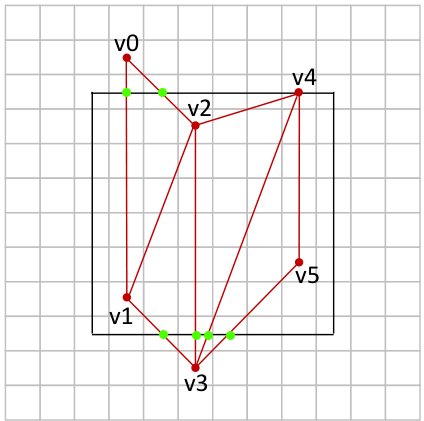      {width=40%}

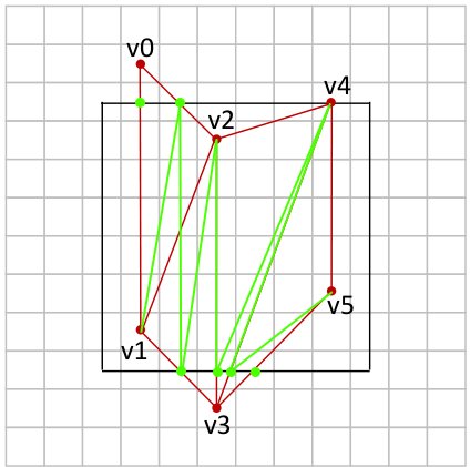
    • \c{How can this new result be expressed as a triangle strip? (Try to be as efficient as possible)}

      The only way to get this to be represented as a triangle strip is to change around the some of the existing lines. Otherwise, the order of the vertices prevents the exact same configuration from working.

      See below for a working version (only consider the green lines, ignore the red lines):

      {width=40%}

    • \c{How many triangles will be encoded in the clipped triangle strip?}

      Based on the image above, 8 triangles will be used.

Ray Tracing vs Scan Conversion

11. \c{(8 points) List the essential steps in the scan-conversion (raster graphics) rendering pipeline, starting with vertex processing and ending with the assignment of a color to a pixel in a displayed image. For each step briefly describe, in your own words, what is accomplished and how. You do not need to include steps that we did not discuss in class, such as tessellation (subdividing an input triangle into multiple subtriangles), instancing (creating new geometric primitives from existing input vertices), but you should not omit any steps that are essential to the process of generating an image of a provided list of triangles.}

    The most essential steps in the scan-conversion process are:

    • First, the input is given as a bunch of geometries. This includes triangles and quads. Spheres aren't really part of the primitives, not sure why historically but I can imagine it makes operations like clipping monstrously more complex.

    • Then, vertices of the geometries are passed to vertex shaders, which are custom user-defined scripts that are run in parallel on graphics hardware that are applied to each individual vertex. This includes things like transforming it through coordinate systems (world coordinates vs. camera coordinates vs. normalized coordinates) in order for the rasterizer to be able to go through and process all of the geometries quickly.

    • Clipping is done as an optimization to reduce the amount of things outside the viewport that needs to be rendered. There are different clipping algorithms available, but they all typically break down triangles into smaller pieces that are all contained within the viewport. Culling is also done to remove faces that aren't visible and thus don't need to be rendered.

    • The rasterizer then goes through and gives pixels colors based on which geometries contain them. This includes determining which geometries are in front of others, usually done using a z-buffer. When a z-buffer is used, the color of the closest object is stored and picked. During this process, fragment shaders also influence the output. Fragment shaders are also custom user-defined programs running on graphics hardware, and can modify things like what color is getting output or the order of the depth buffer based on various input factors.

12. \c{(6 points) Compare and contrast the process of generating an image of a scene using ray tracing versus scan conversion. Include a discussion of outcomes that can be achieved using a ray tracing approach but not using a scan-conversion approach, or vice versa, and explain the reasons why and why not.}

    With ray tracing, the process of generating pixels is very hierarchical. The basic ray tracer was very simple, but the moment we even added shadows, there were recursive rays that needed to be cast, not to mention the jittering. None of those could be parallelized with the main one, because in order to even figure out where to start, you need to have already performed a lot of the calculations. (For my ray tracer implementation, I already parallelized as much as I could using the work-stealing library rayon)

    But with scan conversion, the majority of the transformations are just done with matrix transformations over the geometries, which can be performed completely in parallel with minimal branching (only depth testing is not exactly) The rasterization process is also massively parallelizable. This makes it faster to do on GPUs which are able to do a lot of independent operations.